by DAH Buckley · 2014 · Cited by 1 — Magnetic Cataclysmic Variables (mCVs) are short period (~1.3 – 10h) close binary stars with an accreting magnetic white dwarf primary [1,2]. The bulk of the
124 KB – 6 Pages
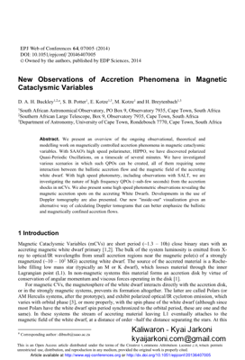
PAGE – 1 ============
New Observations of Accretion Phenomena in Magnetic Cataclysmic Variables D. A. H. Buckley 1,2, a , S. B. Potter 1 , E. Kotze 1,3 , M. Kotze 1 and H. Breytenbach 1,3 1 South African Astronomical Observatory, PO Box 9, Observatory 7935, Cape Town, South Africa 2 Southern African Large Telescope, Box 9, Observatory 7935, Cape Town, South Africa 3 Department of Astronomy, University of Cape Town, Rondebosch 7770, Cape Town, South Africa Abstract. We present an overview of the ongoing observational, theoretical and modelling work on magnetically controlled accretion phenomena in magnetic cataclysmic variables. With SAAO’s high speed polarimeter, HIPPO, we have discovered polarized Quasi-Periodic Oscillations, on a timescale of several minutes. We have investigated various scenarios in which such QPOs can be created, all of them requiring some interaction between the ballistic accretion flow and the magnetic field of the accreting white dwarf. With high speed photometry, including observations with SALT, we are investigating the nature of high frequency QPOs (~sub-few seconds) from the accretion shocks in mCVs. We also present some high speed photometric observations revealing the magnetic accretion spots on the accreting White Dwarfs. Developments in the use of Doppler tomography are also presented. Our new “inside-out” visualization gives an alternative way of calculating Doppler tomograms that can better emphasize the ballistic and magnetically confined accretion flows. 1 Introduction Magnetic Cataclysmic Variables (mCVs) are short period (~1.3 10h) close binary stars with an accreting magnetic white dwarf primary [1 ,2 ]. The bulk of the system luminosity is emitted from X- ray to optical/IR wavelengths from small accretion regions near the magnetic pole(s) of a strongly magnetized (~10 10 2 MG) accreting white dwarf. The source of the accreted material is a Roche- lobe filling low mass star (typically an M or K dwarf), which looses material through the inner Lagrangian point (L1). In non-magnetic systems this material forms an accretion disk by virtue of conservation of angular momentum and viscous forces operating in the disk [1] . For magnetic CVs, the magnetosphere of the white dwarf interacts directly with the accretion disk, or in the strongly magnetic systems, prevents its formation altogether. The latter are called Polars (or AM Herculis systems, after the prototype), and exhibit polarized optical/IR cyclotron emission, which varies with orbital phase [3 ], or more properly, with the spin phase of the white dwarf (although since most Polars have the white dwarf spin period synchronized to the orbital period, these are one and the same) . In these systems the stream of accreting material leaving L1 eventually attaches to the magnetic field of the white dwarf, at a distance of order ~half the distance separatin g the stars. At this a Corresponding author : dibnob@saao.ac.za DOI:10.1051 / C Ownedbytheauthors,publishedbyEDPSciences,2014 , / 07005 (2014) 201 64 epjconf EPJ WebofConferences 46407005 This is an Open Access article distri buted under the terms of the Creative Commons Attribution License 2 . 0, which permits unrestricted use, dist ribution, and reproduction in any medium, provi ded the original work is properly cited. Article available athttp://www.epj-conferences.orgorhttp://dx.doi.org/10.1051/epjconf/20136407005
PAGE – 2 ============
point the magnetic forces overwhelm the ballistic forces and the matter is constrained to follow the magnetic ecomes collimated into a cylindrical accretion column and eventually reaches supersonic velocities, causing a stand- off shock to forms where most of the gravitational potential energy is released as radiation. Accretion may occur on one or both poles, depending on the orientation of the magnetic dipole (see Fig. 1, left) . However the accretion rate may be different for the two poles due to a more or less favourable orientation for a particular pole to accrete efficiently. For the weaker field asynchronous system, termed Intermediate Polars (IPs; sometime also referred to as DQ Herculis stars), the magnetosphere disrupts the inner portion of the accretion disk near the Aflvén radius, and the accretion flow then follows the field lines in a curtain-like structure, extended in azimuth [4 ]. Due to the disc symmetry, the accretion curtains are present for both magnetic poles, resulting in arc-like accretion regions near the white dwarf poles, akin to the auroral ovals on the Earth and Jupiter. There is evidence in some IPs that some fraction of the accre tion stream from L1 follows a ballistic trajectory through the disk, penetrating to the magnetosphere, rather outer edge. This can lead to direct stream accretion, modulated at the orbit-spin beat period (i.e. the synodic period). In at least one case (the system V2400 Oph) all of the accretion is from the stream, resulting in the X-rays varying at the beat period [5 ]. Figure 1. Models for accretion in magnetic CVs. Left: single pole accretion in a Polar. Right: combination of accretion from a disc and a stream in an Intermediate Polar. The emission components in mCVs include hard (>10 20 keV) thermal bremsstrahlung X-rays from the accretion shock, just above the white dwarf surface. A certain fraction of this radiation maybe -rays, UV and optical radiation, a component particularly prevalent in Polars. In many systems bury themselves the kinetic and potential energy and produce a significant soft X-ray/extreme UV component . One of the dominant shock cooling mechanisms is cyclotron emission, usually dominating at optical-IR wavelengths, resulting from spiralling electrons in the strong magnetic field. This emission is strongly linearly and circularly percent . 2 Observing Magnetic CVs at SAAO There is a long tradition of observing mCVs at the SAAO, starting with the pioneering polarimetry observations in the mid-1980s of Polars [6] and extending to high speed photometry and spectroscopy during the ROSAT era [7]. These observations were primarily done with a variety of modest aperture telescopes (0.75m to 1.9m). With the advent of the 10-m class Southern African Large Telescope (SALT; [8]), plus the development of new instrumentation on the smaller SAAO telescopes [9,10] , this work has expanded to take advantage of these new facilities. For SALT the major advance is the large aperture coupled with fast frame transfer CCD detectors for both spectroscopy and photometry, and in the near future, spectropolarimetry. For the other SAAO telescopes, we have a new two- channel photopolarimeter, HIPPO [8], plus two high speed EM-CCD cameras, SHOC 1 & 2 [10]. HIPPO has improved our polarimetric capabilities, with improved efficiency and simultaneous measurements possible in two band-passes. The SHOC cameras allow high time resolution EPJ Web of Conferences EPJ Web of Conferences
PAGE – 3 ============
photometry (down to a ~10 ms ) . In this paper we describe some of the recent observational highlights using these facilities to further our understanding of the accretion processes in mCVs. 2.1 Eclipse Observations of Polar Accretion Hot Spots In eclipsing Polars, the size, structure and location of the accretion regions on the white dwarf can be determined from sufficiently high time resolution (sub-second) photometry. Time resolved spectropolarimetry can also assist in determining the magnetic field strength and geometry and help in probing the characteristics of the cyclotron emitting regions through model fitting. The SALT high-speed CCD camera, SALTICAM, has been used to make high time resolution (down to ~80 ms) photometry of eclipsing Polars. In Figure 2 we show an eclipse egress light curve of data sampling [11]. The intensity steps are due to the progressive re-appearance of two accretion hot-spots near the magnetic poles of the magnetic white dwarf, which take ~1.5 s to be uncovered. The se data have been fitted with a model based on the likely masses of the component stars, as derived from the eclipse parameters and orbital period (1.45h), plus the orbital inclination of the system ( i ) and the co-latitudes of the accretion spots ( 1 and 2 ). Figure 2. Left: SALTICAM high time resolution (~0.1sec samples) eclipse egress observation of FL Cet with model fit. Right: The model for the positions of the accretion regions on the white dwarf [11] . 2.2 Quasi -Periodic Oscillations in Polar Accretion Columns Optical quasi-periodic intensity variations at typically ~1Hz have been detected in some in Polars (e.g. [ 12 ]) and are commonly attributed to plasma oscillations in the magnetically confined accretio n columns. Some suggestions have been made that different parts of the accretion column are magnetically isolated from each other. The typical QPO frequency is thought to be related to the physical parameters, particularly the shock height, inside the accretion column (or sub- co lumns) and therefore the exact characterisation of the QPO properties (e.g. the Q-number, amplitude, period) depends on the sum of the contributions of each sub-column, each with its own potentially varying parameters (e.g. magnetic field strength and fractional mass accretion rate). A systematic program to search for QPOs in Polars, including in newly discovered systems, has re cently started at SAAO. This program utilizes the SHOC instruments, which have much higher QEs (~80%) compared to the PMTs used in previous studies (e.g. [ 12 ]). Our eventual aim is to complete a systematic study of the QPO phenomena in a variety of polars with different physical attributes, for example low and high field systems , asynchronous systems , two-pole accretors , low and high mass systems , low and high accretion rate systems . This work will hopefully lead to a better understanding of the physics underlying the QPOs, taking the study from purely phenomenological to one based on quantitative physical parameters. In conjunction with this observational program, we expect that the experimental results from a parallel program by our collaborators of simulating accretion columns in the laboratory will yield further relevant insights. PhysicsattheMagnetosphericBoundary
PAGE – 4 ============
2.3 Polarized Quasi-Periodic Oscillations in Polars The HIPPO polarimeter was used to do photopolarimetry of the Polar IGR J14536 5522 (=Swift J1453.4 5524) on the SAAO 1.9-m telescope [9 ]. These observations revealed prominent QPOs in both intensity and circular polarized flux, at a typical timescale of ~300 360s. These long period QPOs must therefore be associated with the cyclotron emission region, although they are not detected at all orbital phases, as can be seen in the trailed periodogram, in the second panel from the top in Figure 3. A possible explanation is the preferential viewing of a single magnetic a certain phase interval (~0.0 0.3), which reduces the incoherent flickering that usually results from the superposition of oscillations arising from numerous accretion tubes. Figure 3. HIPPO observations of the Polar IGR J14536 5522 have revealed QPOs in the circularly polarized flux [9] . The upper two panels show the circular polarization and the associated trailed peridodogram, respectively, over the orbit, while the lower three panels focus on the polarized QPOs in the phase interval ~0.05 0.30. 2.4 New – Doppler tomography [13] is a technique which uses the information contained in Doppler-shifted spectra (emission lines, in the case of CVs) as a function of orbital phase to calculate the strength of emission as a function of velocity. The technique produces velocity maps (Doppler tomograms) which have an inverted appearance in velocity space with respect to the real spatial direction. The high velocity regions are seen at the edge of the maps, whereas physically these regions are usually close to the accreting white dwarf, which is close to the centre of mass of the system. We (EK & SBP) have recently devised – – rectify the inverted appearance in velocity space. The aim is to increase the ease of interpretation by producing tomograms that are visually more intuitive. Since we found that the circularly symmetric velocity profile of a Doppler tomogram is more conducive to circularly symmetric transformations in the polar coordinate system, we opted to first convert the traditional Cartesian velocity coordinates to polar velocity coordinates. The velocity magnitude , v , increases as a linear function of distance from the origin, with a direction given by the polar angle, . The inside – out velocity space is obtained by transposing the zero velocity origin of the normal tomogram to the outer diameter dotted circle in the inside – out map. In Figure 4 velocity profile overlays are shown in both tomograms for the secondary star (solid oval in the upper part of each), a single-particle ballistic trajectory emanating from L1 (solid curved line), with small circles marking every 10 azimuthal degrees along the ballistic stream. The EPJ Web of Conferences
PAGE – 5 ============
approximately – free-fall velocities along magnetic field lines of a dipole. The straight dotted lines connect the points on the ballistic stream to the appropriate magnetic field like which intersect it, and indicates the discontinuous velocity change of particles moving from a purely ballistic to a magnetic trajectory. In the inside-out tomogram the ballistic stream now curves inwards as it accelerates towards the white dwarf. The secondary star in the inside-out tomogram appears upside down because it is orbiting as a solid body. The origin of the normal tomogram is the centre of mass of the system, by definition with – now projects to the outer dotted circle. Likewise, Keplerian disc motion, shown at an arbitrary radius as the outer dotted circle in the normal tomogram, now projects to the small er – Figure HeII 4686Å Doppler tomograms of the Polar V834 Cen taken on the SAAO 1.9m telescope [14] were derived using the method of Spruit [15]. The top left and bottom right panels show the input trailed spectra and reconstructed trailed spectra, respectively. top right – (bottom left) tomograms are shown for comparison. 4: PhysicsattheMagnetosphericBoundary
PAGE – 6 ============
The – map shows emission from material with velocities intermediate between low orbital ve locity and ballistic free-fall. Clearly the rendering of Doppl – improves the discrimination of the different emission components and provides a more intuitive presentation. References [1] Warner, B., Cataclysmic Variable S tar s (Cambridge University Press, 1995) [2] Hellier, C., Cataclysmic Variable Stars: how and why they vary (Springer, 2001) [3] Cropper, M., Space Sci. Rev. 54 , 195 (1990) [4] Patterson, J., PASP 106 , 209 (1994) [5] Buckley, D.A.H., et al., MNRAS 287 , 117 (1997) [6] Cropper, M., MNRAS 212 , 709 (1985) [7] Buckley, D.A.H., Astrophys. & Space Sci. 230 , 131 (1995) [8] Buckley, D.A.H., Swart, G., Meiring, J.G., SPIE 6967 , 69670z (2006) [9] Potter, S.B, et al. , MNRAS 412 , 1161 (2010) [10] Coppejans, R. , et al. , PASP 125 , 976 (2013). [11] et al. , MNRAS 372 , 151 (2006) [12] Larsson, S., A&A 217 , 416 (1989). [13] Marsh T., Horne K., MNRAS 235 , 269 (1988). [14] Potter, S.B., Romero-Colmenero, E., Watson, et al., MNRAS 348 , 316 (2004). [15] Spruit, H. C., arXiv:astro-ph/9806141 (1998) EPJ Web of Conferences
124 KB – 6 Pages