Aug 25, 2009 — Absorption is used to separate gas mixtures, remove impurities, or recover valuable chemicals. The operation of removing the absorbed solute.
8 pages
91 KB – 8 Pages
PAGE – 1 ============
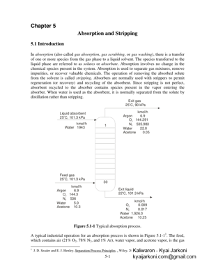
5-1 Chapter 5 Absorption and Stripping 5.1 Introduction In absorption (also called gas absorption , gas scrubbing , or gas washing ), there is a transfer of one or more species from the gas phase to a liqu id solvent. The species transferred to the liquid phase are referred to as solutes or absorbate . Absorption involves no change in the chemical species present in the system. Absorption is used to separate gas mixtures, remove impurities, or recover valuable chemicals. The oper ation of removing the absorbed solute from the solvent is called stripping . Absorbers are normally used with strippers to per mit regeneration (or recovery) and recycling of the abs orbent. Since stripping is not perfect, absorbent recycled to the absorber contains species present in the vapor entering the absorber. When water is used as the absorbent, it i s normally separated from the solute by distillation rather than stripping. 130 Exit gas 25C, 90 kPa o kmol/h O 0.009 N 0.017 Water 1,926.0 Acetone 10.25 22Liquid absorbent 25C, 101.3 kPa o kmol/h Water 1943 Feed gas 25C, 101.3 kPa oExit liquid 22C, 101.3 kPa o kmol/h Argon 6.9 O 144.3 N 536 Water 5.0 Acetone 10.3 22 kmol/h Argon 6.9 O 144.291 N 535.983 Water 22.0 Acetone 0.05 22 Figure 5.1-1 Typical absorption process. A typical industrial operation for an absorption pr ocess is shown in Figure 5.1-1 1. The feed, which contains air (21% O 2, 78% N 2, and 1% Ar), water vapor, and acetone vapor, is th e gas 1 J. D. Seader and E. J. Henley, Separation Process Principles , , Wiley, 2006, pg. 194
PAGE – 2 ============
5-2 leaving a dryer where solid cellulose acetate fiber s, wet with water and acetone, are dried. Acetone is removed by a 30-tray absorber using wate r as the absorbent. The percentage of acetone removed from the air stream is 10.25 10.3 ×100 = 99.5% Although the major component absorbed by water is a cetone, there are also small amounts of oxygen and nitrogen absorbed by the water. Water is also stripped since more water appears in the exit gas than in the feed gas. The temperatu re of the exit liquid decreases by 3 oC to supply the energy of vaporization needed to strip t he water. This energy is greater than the energy of condensation liberated from the absorptio n of acetone. Three approaches have generally been employed to de velop equations used to predict the performance of absorbers and absorption equipment: mass transfer coefficients, graphical solution, and absorption factor. The use of mass tr ansfer coefficient is covered in Chapter 2.2. The graphical solution is simple to use for on e or two components and provides explicit graphical presentation of the interrelationships of the variables and parameters in an absorption process. However the graphical technique becomes very tedious when several solutes are present and must be considered. The abs orption factor approach can be utilized either for hand or computer calculation. Absorption and stripping are conducted mainly in packed columns and plate columns (trayed tower) as shown in Figure 5.1-2. Packed column 2 Plate column 3 Figure 5.1-2 Equipment for absorption and stripping. 2 www.mikropul.com/products/wscrubber/packed.htm (Aug. 25 2009) 3 http://www.cgscgs.com/ga_tt.htm (Aug. 25 2009)
PAGE – 3 ============
5-3 5.2 Single-Component Absorption Most absorption or stripping operations are carried out in counter current flow processes, in which the gas flow is introduced in the bottom of t he column and the liquid solvent is introduced in the top of the column. The mathematic al analysis for both the packed and plated columns is very similar. L xtA,t L xbA,b VytA,t V ybA,b L V Figure 5.2-1 Countercurrent absorption process. The overall material balance for a countercurrent a bsorption process is Lb + Vt = Lt + Vb (5.2-1) where V = vapor flow rate L = liquid flow rate t, b = top and bottom of tower, respectively The component material balance for species A is LbxA,b + Vt yA,t = LtxA,t + Vb yA,b (5.2-2) where yA = mole fraction of A in the vapor phase xA = mole fraction of A in the liquid phase For some problems, the use of solute-free basis can simplify the expressions. The solute-fre e concentrations are defined as: AX = 1AAxx-= mole fraction of A in the liquid mole fraction of non-A components in the liquid (5.2-3a) AY = 1AAyy-= mole fraction of A in the vapor mole fraction of non-A components in the vapor (5.2-3b) If the carrier gas is completely insoluble in the s olvent and the solvent is completely nonvolatile, the carrier gas and solvent rates rema in constant throughout the absorber. Using
PAGE – 4 ============
5-4 Lto denote the flow rate of the nonvolatile and Vto denote the carrier gas flow rate, the material balance for solute A becomes L,Ab X + V,At Y = L,At X + V,Ab Y (5.2-4) or ,At Y = LV,At X + ,,Ab Ab LX YV – (5.2-5) The material balance for solute A can be applied to any part of the column. For example, the material balance for the top part of the column is ,At Y = LV,At X + AALX YV – (5.2-6) In this equation, AXand AYare the mole ratios of A in the liquid and vapor ph ase, respectively, at any location in the column includi ng at the two terminals. Equation (5.2-6) is called the operation line and is a straight line wi th slope LV when plotted on AX-AYcoordinates. The equilibrium relation is frequently given in ter ms of the Henry™s law constant which can be expressed in many different ways: PA = CA = mx A = Kx A (5.2-7) In this equation, PA is the partial pressure of species A over the solu tion and CA is the molar concentration with units of mole/volume. The Henry™ s law constant and m have units of pressure/molar concentration and pressure/mole frac tion, respectively. K is the equilibrium constant or vapor-liquid equilibrium ratio. Table 5 .2-1 list Henry™s law constant m for various gases in water. Table 5.2-1 Henry™s Law constant for Gases in water 4 ( m×10 -4 atm/mole fraction) T(oC) CO 2 CO C 2H6 C2H4 He H 2 H2S CH 4 N2 O2 0 10 20 30 40 0.0728 0.104 0.142 0.186 0.233 3.52 4.42 5.36 6.20 6.96 1.26 1.89 2.63 3.42 4.23 0.552 0.768 1.02 1.27 12.9 12.6 12.5 12.4 12.1 5.79 6.36 6.83 7.29 7.51 0.0268 0.0367 0.0483 0.0609 0.0745 2.24 2.97 3.76 4.49 5.20 5.29 6.68 8.04 9.24 10.4 2.55 3.27 4.01 4.75 5.35 Example 5.2-1 . 5 ————————————————— ——————————- A solute A is to be recovered from an inert carrier gas B by absorption into a solvent. The gas entering into the absorber flows at a rate of 500 k mol/h with yA = 0.3 and leaving the absorber with yA = 0.01. Solvent enters the absorber at the rate of of 1500 kmol/h with xA = 4 Geankoplis, C.J., Transport Processes and Separati on Process Principles , 4 th edition, Prentice Hall, 2003, pg. 988 5 Hines, A. L. and Maddox R. N., Mass Transfer: Fund amentals and Applications, Prentice Hall, 1985, pg. 255
PAGE – 5 ============
5-5 0.001. The equilibrium relationship is yA = 2.8 x A. The carrier gas may be considered insoluble in the solvent and the solvent may be con sidered nonvolatile. Construct the x-y plots for the equilibrium and operating lines using both mole fraction and solute-free coordinates. Solution ————————————————— ————————————– The flow rates of the solvent and carrier gas are g iven by L= Lt(1 – xA,t ) = 1500(1 – 0.001) = 1498.5 kmol/h V = Vb(1 – yA,b ) = 500(1 – 0.3) = 350 kmol/h The concentration of A in the solvent stream leavin g the absorber can be determined from the following expressions: xA,b = bbMoles A in Moles A in + LLL Moles of A in Lb = Moles of A in Lt + Moles of A in Vb – Moles of A in Vt Moles of A in Lb = 1500×0.001 + 500×0.3 – Moles of A in Vt yA,t = ttMoles A in Moles A in + VVV 0.01 = ttMoles A in Moles A in + 350 VV Moles of A in Vt = 350×0.01/(1 – 0.01) = 3.5354 kmol/h Moles of A in Lb = 1.500 + 150 – 3.5354 = 147.965 kmol/h xA,b = bbMoles A in Moles A in + LLL = 147.965 147.965 + 1498.5 = 0.0898 For the solute free basis: AX = 1AAxx-, AY = 1AAyy- ,At X = ,,1At At xx-= 0.0010 10.0010 – = 0.0010 ,Ab X = ,,1Ab Ab xx-= 0.0898 10.0898 – = 0.0987
PAGE – 6 ============
5-6 ,At Y = ,,1At At yy-= 0.010 10.010 – = 0.0101 ,Ab Y = ,,1Ab Ab yy-= 0.30 10.30 – = 0.4286 The equilibrium curves in both mole fraction and so lute-free coordinates are calculated from the following procedures: 1) Choose a value of xA between 0.001 and 0.10 2) Evaluate the corresponding AX = 1AAxx- 3) Evaluate yA = 2.8 x A 4) Evaluate the corresponding AY = 1AAyy- The operating lines in both mole fraction and solut e-free coordinates are calculated from the following procedures: 1) Choose a value of xA between 0.001 and 0.0898 2) Evaluate the corresponding AX = 1AAxx- 3) Evaluate AY = LVAX + ,,Ab Ab LX YV – 4) Evaluate the corresponding yA = 1AAYY+ The following Matlab codes plot the equilibrium and operating lines in both mole fraction and solute-free coordinates. ——————————————- % Example 5.2-1 xe=linspace(0.001,0.1); ye=2.8*xe; Xe=xe./(1-xe);Ye=ye./(1-ye); x=linspace(0.001,0.0898); Lbar=1498.5;Vbar=350; X=x./(1-x);Xb=.0898;Yb=0.4286; LoV=Lbar/Vbar; Y=LoV*X+Yb-LoV*Xb; y=Y./(1+Y); plot(xe,ye,x,y,’–‘) legend(‘Equilibrium curve’,’Operating line’,2) xlabel(‘x’);ylabel(‘y’) Title(‘Equilibrium and Operating lines on mole frac tion coordinates’) figure(2) plot(Xe,Ye,X,Y,’–‘) legend(‘Equilibrium curve’,’Operating line’,2)
PAGE – 8 ============
5-8 YXYbYtXtXbYbYbYtYtXtXtXbXbYcXc(A) (B) (C) Figure 5.2-2 Limiting conditions for absorption process. The driving force for mass transfer becomes zero wh enever the operating line intersects or touches the equilibrium curve. This limiting condit ion represents the minimum solvent rate to recover a specified quantity of solute or the solve nt rate required to remove the maximum amount of solute. In Figure 5.2-2A, the intersectio n of the equilibrium and operating lines occurs at the bottom of the absorber. This conditio n defines the minimum solvent rate to recover a specified quantity of solute. This minimu m solvent rate can be calculated from the following expression: min LV = bt bt YY XX – – (5.2-8a) In Figure 5.2-2B, the intersection of the equilibri um and operating lines occurs at the top of the absorber. This condition represents the solvent rate required to remove the maximum amount of solute. This solvent rate can be calculat ed from the following expression: max LV = bt bt YY XX – – (5.2-8b) Equation (5.2-8b) is exactly the same as Eq. (5.2-8 a) except in this case the bottom compositions are fixed so that the maximum slope of the operating line occurs when the operating line intersects the equilibrium curve at the top of the column. Figure 5.2-2C shows the case when the operating lin e becomes tangent to the equilibrium curve. The minimum liquid-to-vapor ratio for this c ase can be determined from min LV = ct ct YY XX – – (5.2-9) In this equation, cY and cX are the coordinates of the tangent point.
91 KB – 8 Pages